The emergence of heat and humidity too severe for human tolerance.

Abstract

Humans’ ability to efficiently shed heat has enabled us to range over every continent, but a wet-bulb temperature (TW) of 35°C marks our upper physiological limit, and much lower values have serious health and productivity impacts. Climate models project the first 35°C TW occurrences by the mid-21st century. However, a comprehensive evaluation of weather station data shows that some coastal subtropical locations have already reported a TW of 35°C and that extreme humid heat overall has more than doubled in frequency since 1979. Recent exceedances of 35°C in global maximum sea surface temperature provide further support for the validity of these dangerously high TW values. We find the most extreme humid heat is highly localized in both space and time and is correspondingly substantially underestimated in reanalysis products. Our findings thus underscore the serious challenge posed by humid heat that is more intense than previously reported and increasingly severe.

 

INTRODUCTION

Humans’ bipedal locomotion, naked skin, and sweat glands are constituents of a sophisticated cooling system (1). Despite these thermoregulatory adaptations, extreme heat remains one of the most dangerous natural hazards (2), with tens of thousands of fatalities in the deadliest events so far this century (3, 4). The additive impacts of heat and humidity extend beyond direct health outcomes to include reduced individual performance across a range of activities, as well as large-scale economic impacts (5–7). Heat-humidity effects have prompted decades of study in military, athletic, and occupational contexts (8, 9). However, consideration of wet-bulb temperature (TW) from the perspectives of climatology and meteorology began more recently (10, 11).

While some heat-humidity impacts can be avoided through acclimation and behavioral adaptation (12), there exists an upper limit for survivability under sustained exposure, even with idealized conditions of perfect health, total inactivity, full shade, absence of clothing, and unlimited drinking water (9, 10). A normal internal human body temperature of 36.8° ± 0.5°C requires skin temperatures of around 35°C to maintain a gradient directing heat outward from the core (10, 13). Once the air (dry-bulb) temperature (T) rises above this threshold, metabolic heat can only be shed via sweat-based latent cooling, and at TW exceeding about 35°C, this cooling mechanism loses its effectiveness altogether. Because the ideal physiological and behavioral assumptions are almost never met, severe mortality and morbidity impacts typically occur at much lower values—for example, regions affected by the deadly 2003 European and 2010 Russian heat waves experienced TW values no greater than 28°C (fig. S1). In the literature to date, there have been no observational reports of TW exceeding 35°C and few reports exceeding 33°C (9, 11, 14, 15). The awareness of a physiological limit has prompted modeling studies to ask how soon it may be crossed. Results suggest that, under the business-as-usual RCP8.5 emissions scenario, TW could regularly exceed 35°C in parts of South Asia and the Middle East by the third quarter of the 21st century (14–16).

Here, we use quality-assured station observations from HadISD (17, 18) and high-resolution reanalysis data from ERA-Interim (19, 20), verified against radiosondes and marine observations (see the Supplementary Materials) (21, 22), to compute TW baseline values, geographic patterns, and recent trends. Uncertainties in TW from station data due to instrumentation and procedures are on the order of 0.5° to 1.0°C in all regions considered, an important consideration for proper interpretation of the results. Our approach of using TW and sea surface temperature (SST) observations as guidance for future TW projections offers a different line of evidence from previous research that used coupled or regional models without explicitly including historical station data.

RESULTS

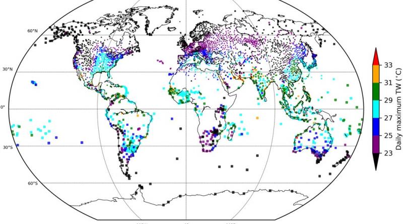
Our survey of the climate record from station data reveals many global TW exceedances of 31° and 33°C and two stations that have already reported multiple daily maximum TW values above 35°C. These conditions, nearing or beyond prolonged human physiological tolerance, have mostly occurred only for 1- to 2-hours’ duration (fig. S2). They are concentrated in South Asia, the coastal Middle East, and coastal southwest North America, in close proximity to extraordinarily high SSTs and intense continental heat that together favor the occurrence of extreme humid heat (2, 14). Along coastlines, the marine influence is manifest via anomalous onshore low-level winds during midday and afternoon hours, and these wind shifts can cause rapid dew point temperature (Td) increases in arid and semiarid coastal areas (figs. S3 to S9). Regionally coherent observational evidence supports these intense values: Of the stations along the Persian Gulf coastline with at least 50% data availability over 1979 to 2017, all have a historical 99.9th percentile of TW (the value exceeded roughly 14 times in 39 years) above 31°C (Fig. 1; see fig. S1 for the all-time maximum). In the ERA-Interim reanalysis, the highest values are similarly located over the Persian Gulf and immediately adjacent land areas, as well as parts of the Indus River Valley (fig. S10). The spatiotemporal averaging inherent in reanalysis products causes ERA-Interim to be unable to represent the short durations and small areas of critical heat stress, causing its extreme TW values to be substantially lower than those of weather stations across the tropics and subtropics (fig. S11). In the Persian Gulf and adjacent Gulf of Oman, these differences are consistently in the range of −2° to −4°C (fig. S12). Larger bias but similar consistency is present along the eastern shore of the Red Sea, presenting a basis for future studies examining the reasons for this behavior, as well as further comparisons between station and reanalysis data.

Other >31°C hotspots in the weather station record emerge through surveying the globally highest 99.9th TW percentiles: eastern coastal India, Pakistan and northwestern India, and the shores of the Red Sea, Gulf of California, and southern Gulf of Mexico (Fig. 1). All are situated in the subtropics, along coastlines (typically of a semienclosed gulf or bay of shallow depth, limiting ocean circulation and promoting high SSTs), and in proximity to sources of continental heat, which together with the maritime air comprise the necessary combination for the most exceptional TW (11). That subtropical coastlines are hotspots for heat stress has been noted previously (23, 24); our analysis makes clear the broad geographic scope but also the large intraregional variations (Fig. 1). Western South Asia stands as the main exception to this coastline rule, likely due to the efficient inland transport of humid air by the summer monsoon together with large-scale irrigation (15, 25). Tropical forest and oceanic areas generally experience TW no higher than 31° to 32°C, perhaps a consequence of the high evapotranspiration potential and cloud cover, along with the greater instability of the tropical atmosphere. However, more research is needed on the thermodynamic mechanisms that prevent these areas from attaining higher values.

Steep and statistically significant upward trends in extreme TW frequency (exceedances of 27°, 29°, 31°, and 33°C) and magnitude are present across weather stations globally (Fig. 2). Each frequency trend represents more than a doubling of occurrences of the corresponding threshold between 1979 and 2017. Trends in ERA-Interim are strongly correlated with those of HadISD but are smaller for the highest values (Fig. 2), consistent with ERA-Interim’s underestimation of extreme TW that is largest for the most extreme conditions (fig. S11). We also find a sharp peak in the number of global TW = 27°C and TW = 29°C extremes during the strong El Niño events of 1998 and 2016. Linearly detrending this global-TW-extremes time series reveals that the El Niño–Southern Oscillation (ENSO) correlation is largest for TW values that are high but not unusual (~27° to 28°C) across the tropics and subtropics (fig. S13). Further work is necessary to test to what extent this relationship may be related to the effect of ENSO on hydrological extremes at the global scale, on tropospheric-mean temperatures, or on SSTs in particular basins, and the implications of these effects for TW predictability (26, 27). Overall, TW extremes in the tropics largely correspond on an interannual basis to mean TW (fig. S14), indicating that climate forcings and modes of internal variability resulting in mean temperature shifts can be expected to modulate tropical TW extremes. This is the case in the subtropics as well, although to a somewhat lesser extent.

We also observe modulation on a seasonal scale, by considering as an illustrative example the South Asian monsoon region. There, the timing of peak TW varies with the advance of the summer monsoon (15). Splitting South Asia into “early monsoon” and “late monsoon” subregions, we find that the number of TW extremes is largest around the time of the local climatological monsoon onset date (Fig. 3). Although equivalent extreme values of TW are possible before, during, and after the monsoon rains in any given year, they are of a different character; especially in the northern and western parts of the subcontinent, they become continually moister and have lower dry-bulb temperatures as summer progresses. Across the globe, such temperature and humidity variations occur within a well-defined bivariate space (fig. S15). That these variations are systematically associated with the summer monsoon in South Asia emphasizes the important role of moisture, and of weather systems on synoptic to subseasonal time scales, in controlling extreme TW (15, 28). Our findings underscore the diversity of conditions that can lead to extreme humid heat in the same location at different times, suggesting that impacts adaptation strategies may benefit from taking this recognition into account. Such intraseasonal variability in TW also matters for physiological acclimation, which requires several-day time scales to develop (29); TW character is especially relevant when considering effects on human systems that vary in their sensitivity to humidity and temperature—for example, thermoregulation and energy demand for artificial cooling are strongly affected by TW, whereas the materials that make up the built environment are principally affected by temperature alone (13, 30).

While our analysis of weather stations indicates that TW has already been reported as having exceeded 35°C in limited areas for short periods, this has not yet occurred at the regional scale represented by reanalysis data, which is also the approximate scale of model projections of future TW extremes considered in previous studies (14, 15). To increase the comparability of our station findings with these model projections, we implement a generalized extreme value (GEV) analysis to estimate the amount of global warming from the preindustrial period until TW will regularly exceed 35°C at the global hottest ERA-Interim grid cells, currently all located in the Persian Gulf area (Fig. 4). Complete details of this procedure are in Materials and Methods. In brief, we fit a nonstationary GEV model to the grid cells experiencing the highest TW values, with the GEV location parameter a function of the annual global-mean air-temperature anomaly. This enables us to quantify how much global warming is required for annual maximum TW ≥ 35°C to become at most a 1-in-30-year event at any grid cell. We conduct this analysis solely for grid cells where the nonstationary GEV model is a significantly (P < 0.05) better fit to the annual maximum time series (1979–2017) than a stationary alternative. We then define the temperature of emergence (ToE) as the amount of global warming required until TW ≥35°C is at most a 1-in-30-year event at the ERA-Interim spatiotemporal scale, such that the lowest ToE at any grid cell approximates the first occurrences of TW = 35°C that are widespread and sustained enough to cause serious or fatal health impacts, as estimated from physiological studies (6, 10, 31).

Our method yields a ToE of 1.3°C over the waters of the Persian Gulf (90% confidence interval, 0.81° to 1.73°C) and of 2.3°C for nearby land grid cells (1.4° to 3.3°C) (Fig. 4). Adjusting these numbers for ERA-Interim’s robust Persian Gulf differences of approximately −3°C for extreme TW (fig. S12) supports the conclusion from the station observations that recent warming has increased exceedances of TW = 35°C, but that this threshold has most likely been achieved on occasion throughout the observational record (Fig. 2). The strong marine influence on these values is also apparent in Fig. 1.

To further assess the physical realism of our GEV extrapolation, we additionally examine observed annual maximum (monthly mean) SSTs. An atmospheric boundary layer fully equilibrated with the ocean surface would be at saturation and have the same temperature as the underlying SSTs, meaning that, in principle, 35°C is the lowest SST that could sustain the critical 35°C value of TW in the air above. In reality, equilibrium will not be achieved if air-mass residence times over extreme SSTs are too short, which is more likely if the vertical profile of the atmosphere allows strong surface heating to trigger deep convection (10). Current large-scale SSTs and their trends may therefore provide some guidance as to whether our projections of extreme TW are physically plausible. It is in this context that we note monthly mean SSTs exceeding the 35°C threshold for the first time, reaching 35.2°C in the Persian Gulf in 2017 (Fig. 5). As a result, our GEV projection of large-scale maritime TW ≥ 35°C, for less than 1.5°C warming, appears physically consistent with SST observations at the same scale. Analogous corroboration of station-based TW ≥ 35°C events is provided by point scale, hourly SST and TW across the Persian Gulf from an independent database of marine observations (see the Supplementary Materials) (21), in which we find SSTs have exceeded 35°C in every year since 1979, with ~33% of July to September 2017 observations above this threshold. During the summer of 2017, reports of Persian Gulf over-water TW ≥ 35°C also peaked at ~6% of all TW measurements there.

DISCUSSION

The station-based approach that we take here and the model-based approach taken in previous studies (14–16) represent different methods for obtaining valuable perspective on the genesis and characteristics of global TW extremes. The primary strength of station data is its ability to precisely capture local conditions, but even the best-available station data have limitations, uncertainties, and potential unobserved humidity biases (for example, due to observational procedures, instrumentation type, or siting), as well as highly incomplete spatial coverage (see discussion in the Supplementary Materials) (32, 33). In contrast, reanalysis products and high-resolution regional models satisfy the need for spatiotemporal continuity and consistency and allow analysis of additional variables, but often underestimate extremes (34).

In this study, we demonstrate that efforts to better understand extreme TW would benefit from further close examination, and improved standardization and integration, of station data to alleviate model shortcomings—especially along coasts where TW can vary markedly over small distances and where high-quality humidity data are therefore essential—but that station-based and physical modeling–based approaches are fundamentally complementary. Further research into the origins of extreme-TW biases in gridded products and continued advances in data assimilation would also help enable the development of a more unified approach drawing on all available sources of knowledge. For instance, it is important to understand the treatment of extreme values in reanalyses, and whether false-positive or false-negative rejections might be taking place, particularly as temperature and humidity distributions shift toward ever-higher values. Key multiscale TW processes necessitating closer comparison between observations and models include coastal upwelling, atmospheric convection, land-atmosphere interactions, and atmospheric variability linked to SSTs (28)—for instance, at the hourly, 1- to 10-km scale. Detailed analyses of individual events could help illuminate the unfolding interactions of processes and provide additional investigative power, such as in tracing and forecasting the rapid increases in humidity, which tend to accompany TW extremes (fig. S5), and in assessing the role of topography and land use/land cover in creating apparent TW hotspots (fig. S4). Studies comparing biases and trends in TW and SSTs among reanalyses, models, and regions would be especially beneficial, as would investigation of the sensitivity of extreme-TW projections to historical variability, changes in forcing patterns, and statistical methodologies.

Imminent severe humid heat provides incentive for a broad interdisciplinary research initiative to better characterize health impacts. Increased collection of high-resolution health data, international collaborations with public health experts and social scientists, and dedicated modeling projects would aid in answering questions about how vulnerable populations (such as the elderly, outdoor laborers, and those with preexisting health conditions) will be adversely affected as peak TW advances further into the extreme ranges we consider here. Of particular salience is the need to ascertain how acclimation to high-heat-stress conditions is diminished as the physiological survivability limit is approached. Such efforts may also help resolve the reasons for the paucity of reported mortality and morbidity impacts associated with observed near 35°C conditions (11, 14).

Our findings indicate that reported occurrences of extreme TW have increased rapidly at weather stations and in reanalysis data over the last four decades and that parts of the subtropics are very close to the 35°C survivability limit, which has likely already been reached over both sea and land. These trends highlight the magnitude of the changes that have taken place as a result of the global warming to date. At the spatial scale of reanalysis, we project that TW will regularly exceed 35°C at land grid points with less than 2.5°C of warming since preindustrial—a level that may be reached in the next several decades (35). According to our weather station analysis, emphasizing land grid points underplays the true risks of extreme TW along coastlines, which tends to occur when marine air masses are advected even slightly onshore (14). The southern Persian Gulf shoreline and northern South Asia are home to millions of people, situating them on the front lines of exposure to TW extremes at the edge of and outside the range of natural variability in which our physiology evolved (36). The deadly heat events already experienced in recent decades are indicative of the continuing trend toward increasingly extreme humid heat, and our findings underline that their diverse, consequential, and growing impacts represent a major societal challenge for the coming decades.

MATERIALS AND METHODS

Weather station observations

We use HadISD, version 2.0.1.2017f, which is produced by the Met Office Hadley Centre as a more rigorously quality-controlled version of the National Climatic Data Center Integrated Surface Database (ISD) (17, 18). HadISD results from the implementation of additional data availability and quality control procedures to ISD, including checks on both temperature and Td, the two variables required for computing TW. Because of a lack of good-quality data in the tropics, our conclusions are most reliable in the subtropics and midlatitudes, especially where multiple nearby stations are in agreement. TW uncertainties range from ~0.5°C for the most recent data from North America and Europe to ~1.2°C for the oldest data and that from South Asia, Africa, and Latin America. Data validation is considered in depth in the Supplemental Materials.

We use a MATLAB implementation (37) of the formula of (38) for computing TW. We compute TW daily maxima irrespective of stations’ temporal resolutions, which vary from 1 to 6 hours. TW values are for 2 m above ground level, with station surface pressure calculated from its elevation using a standard atmosphere and an assumed sea-level pressure of 1013 mb. A sensitivity analysis reveals the error in TW owing to this assumption to be on the order of 0.1°C.

We additionally eliminate HadISD station data that fail any one of the following meteorological and climatological tests. Tests are listed in the order implemented, with the fraction of HadISD 31+°C readings removed at each successive step shown in parentheses:

1. A TW extreme occurs in conjunction with a dew point depression of ≤0.5°C (65/10,492).

2. The Td associated with a TW extreme is more than 10°C different from the elevation-adjusted value at the closest grid cell and time step in the ERA-Interim reanalysis (289/10,427).

3. A TW extreme occurring in 1979–1993 is greater than the maximum in 2003–2017 (67/10,138).

4. A TW extreme is followed at any point by at least 1000 consecutive days of missing Td data (365/10,071).

5. A TW extreme occurs on a day when the daily maximum and daily minimum T or Td are identical (53/9706).

6. A TW extreme is more than 7.5°C higher than any other TW value co-occurring in a 7.5° × 7.5° box centered on the station (405/9653).

7. A TW extreme is associated with a Td change of more than 8°C in 1 hour or 12°C in 3 hours (77/9248).

8. A TW extreme is associated with a Td greater than the previously reported, although unofficial, global maximum value of 35°C recorded at Dhahran, Saudi Arabia, on 8 July 2003 (18/9171).

9. A TW extreme occurs during a period with two or more consecutive identical daily maximum TW and Td values (289/9153).

10. A TW extreme before 2001 is higher than any value recorded since 2001 (270/8864).

11. The top five TW extremes at a station all occur within a 365-day period (60/8594).

12. The Td associated with a TW extreme is higher than the 99.5th percentile of the first 5000 days, only at stations where this value is more than 1°C larger than the 99.9th percentile of the last 5000 days (55/8534).

13. The Td associated with a TW extreme is higher than the 99.5th percentile of the last 5000 days, only at stations where this value is more than 6°C larger than the 99.9th percentile of the first 5000 days (362/8479).

14. A TW extreme is associated with a relative humidity of ≥95% (29/8117).

15. A TW extreme occurs on a day when the daily maximum TW takes place before 11:00 a.m. or after 8:00 p.m. local standard time (26/8088).

16. A TW extreme is the all-time maximum at a station and is more than 2°C higher than the next largest value (6/8062).

17. A remaining ≥33°C TW extreme is manually ascertained to be associated with a significant changepoint or not fully supported by gridded humidity and temperature data (508/8056).

Remaining TW = 35°C readings are also closely examined on a subdaily basis so as to ensure validity to the extent possible. We deem valid all other values that pass the above additional quality control measures, beyond the original quality control and homogenization (17, 18). Summaries of the TW = 33°C and 35°C values in the final dataset are given in tables S1 and S2.

Interannual trends are calculated using an ordinary least squares regression, with significance evaluated using a t test on the slope coefficient. Our assessment of extreme TW frequency considers threshold exceedances in 2°C increments from 35° to 27°C, so as to strike a balance between values that are sufficiently distinct from one another while being high enough to remain relevant from an impact perspective.

Marine observations

We use monthly SSTs from the 1° HadISST version 1.1 dataset (20) to assess the physical realism of our GEV extrapolations and use in situ point observations of SST and TW from International Comprehensive Ocean-Atmosphere Data Set (ICOADS) (21) as an independent (versus HadISD) check on the extreme TW values reported at nearby land-based weather stations. Details of these comparisons are provided in the Supplementary Materials.

Marine and vertical profile data

The ICOADS integrated dataset (21) is used as validation of near-surface conditions over water. Radiosondes are from the Integrated Global Radiosonde Archive (22, 39).

GEV modeling of TW extremes in reanalysis data

We fit a GEV distribution to the time series of annual maximum TW from selected grid cells in ERA-Interim, a reanalysis dataset that optimally blends observations with a numerical hindcast and, thus, provides an estimate of the atmospheric state less sensitive to observation error and microclimatic variability (19). While well suited to identifying and extrapolating global trends, it is inevitable in such an approach that decadal temperature trends and other large-scale variability may affect our results modestly.

The cumulative distribution function of the GEV is given by

F(x)=e−[1+к(x−ζ)β]−1к

(1)

The TW quantile for an n-year return period can be evaluated by inverting Eq. 1

F−1(p)=ζ+βк{[−ln (p)]−к−1}

(2)where the location, scale, and shape parameters are denoted ζ, β, and к, respectively. Note that, in our analysis, we use n = 30 (and hence P = 0.967), although we expect different choices of n would not qualitatively affect the results. We estimate these parameters using the method of maximum likelihood, only fitting distributions to series from grid cells whose maximum value over 1979 to 2017 was in the highest 0.1% worldwide (top 119 grid cells), corresponding to a TW threshold of 30.6°C.

We incorporate the effect of global warming on the return period by parameterizing ζ as a function of the annual global mean air temperature anomaly

ζ(⟨T⟩)=α2+α3⟨T⟩

(3)where α₂ and α₃ are the intercept and slope coefficients of a linear regression.

The extent of improvement in this nonstationary model for each grid cell is evaluated using a likelihood ratio test, with test statistic lambda

Λ=2[L(HA)−L(H0)]

(4)where L is the log-likelihood of the nonstationary (subscript A) and stationary (subscript 0) models. Under the null hypothesis (that the nonstationary model is not superior), lambda has a chi-squared distribution with one degree of freedom. Of the 119 grid cells fitted with a GEV distribution, for ~83% of them (99 grid cells), parameterizing zeta as a function of 〈T〉 results in a statistically significant improvement at the P = 0.05 level.

We use the nonstationary model to infer the amount of global warming required for annual maximum TW = 35°C to be at most a 1-in-30-year event. This is calculated by substituting Eq. 3into Eq. 2 and solving for 〈T〉

⟨T⟩=−βк{[−ln(p)]−к−1}+35−α2α3

(5)

Applying Eq. 5 to the 99 grid cells with nonstationary models enables spatially explicit assessments of the amount of global warming required until TW = 35°C should be expected, on average, once per 30-year period at each cell. Here, we have used the HadCRUT4 dataset (version 4.6.0.0) to characterize observed warming (40).

Temperature of TW = 35°C emergence and its uncertainty estimation

The spatially resolved estimates of 〈T〉 from Eq. 5 provide the means for identifying the ToE, which we define as the lowest of the 99 values of 〈T〉 returned by Eq. 5 and which we highlight with vertical dotted lines in Fig. 4. Uncertainty in the ToE is assessed with a 10,000-member bootstrap simulation. We randomly select with replacement 30 years of TW and SST data from within the period 1979–2017, fitting parameters (slope, intercept, shape, and scale for Eq. 5) for each subset. For each bootstrap iteration, we repeat the calculation of the ToE. These 10,000 estimates are then sorted to identify the 5th, 50th, and 95th percentiles; the most likely estimate; and the 90% confidence intervals.

SUPPLEMENTARY MATERIALS

Supplementary material for this article is available at http://advances.sciencemag.org/cgi/content/full/6/19/eaaw1838/DC1

This is an open-access article distributed under the terms of the Creative Commons Attribution-NonCommercial license, which permits use, distribution, and reproduction in any medium, so long as the resultant use is not for commercial advantage and provided the original work is properly cited.

REFERENCES AND NOTES

1. ↵
   1. P. E. Wheeler
   , The thermoregulatory advantages of hominid bipedalism in open equatorial environments: The contribution of increased convective heat loss and cutaneous evaporative cooling. J. Hum. Evol. 21,107–115 (1991).

   CrossRefWeb of ScienceGoogle Scholar

2. ↵
   1. M. Wehner, 
   2. D. Stone, 
   3. H. Krishnan, 
   4. K. AchutaRao, 
   5. F. Castillo
   , The deadly combination of heat and humidity in India and Pakistan in summer 2015. Bull. Amer. Meteorol. Soc. 97, S81–S86 (2016).

   Google Scholar

3. ↵
   1. J.-M. Robine, 
   2. S. L. K. Cheung, 
   3. S. Le Roy, 
   4. H. Van Oyen, 
   5. C. Griffiths, 
   6. J.-P. Michel, 
   7. F. R. Herrmann
   , Death toll exceeded 70,000 in Europe during the summer of 2003. C. R. Biol. 331, 171–178 (2008).

   CrossRefPubMedWeb of ScienceGoogle Scholar

4. ↵
   1. B. A. Revich
   , Heat-wave, air quality and mortality in European Russia in summer 2010: Preliminary assessment. Ekol. Cheloveka Hum. Ecol. , 3–9 (2011).

   Google Scholar

5. ↵
   1. T. K. R. Matthews, 
   2. R. L. Wilby, 
   3. C. Murphy
   , Communicating the deadly consequences of global warming for human heat stress. Proc. Nat. Acad. Sci. U.S.A. 114, 3861–3866 (2017).

   Abstract/FREE Full TextGoogle Scholar

6. ↵
   1. C. Mora, 
   2. B. Dousset, 
   3. I. R. Caldwell, 
   4. F. E. Powell, 
   5. R. C. Geronimo, 
   6. C. R. Bielecki, 
   7. C. W. W. Counsell, 
   8. B. S.Dietrich, 
   9. E. T. Johnston, 
   10. L. V. Louis, 
   11. M. P. Lucas, 
   12. M. M. McKenzie, 
   13. A. G. Shea, 
   14. H. Tseng, 
   15. T. W. Giambelluca, 
   16. L. R. Leon, 
   17. E. Hawkins, 
   18. C. Trauernicht
   , Global risk of deadly heat. Nat. Clim. Change 7, 501–506 (2017).

   Google Scholar

7. ↵
   1. T. Kjellstrom, 
   2. D. Briggs, 
   3. C. Freyberg, 
   4. B. Lemke, 
   5. M. Otto, 
   6. O. Hyatt
   , Heat, human performance, and occupational health: A key issue for the assessment of global climate change impacts. Annu. Rev. Public Health 37, 97–112 (2016).

   Google Scholar

8. ↵

   M. N. Sawka, C. B. Wenger, S. J. Montain, M. A. Kolka, B. Bettencourt, S. Flinn, J. Gardner, W. T. Matthew, M. Lovell, C. Scott, Heat Stress Control and Heat Casualty Management (US Army Research Institute of Environmental Medicine Technical Bulletin 507, 2003).

9. ↵
   1. K. Parsons
   , Heat stress standard ISO 7243 and its global application. Ind. Health 44, 368–379 (2006).

   CrossRefPubMedWeb of ScienceGoogle Scholar

10. ↵
    1. S. C. Sherwood, 
    2. M. Huber
    , An adaptability limit to climate change due to heat stress. Proc. Natl. Acad. Sci. U.S.A. 107, 9552–9555 (2010).

    Abstract/FREE Full TextGoogle Scholar

11. ↵
    1. C. Schär
    , Climate extremes: The worst heat waves to come. Nat. Clim. Change 6, 128–129 (2016).

    Google Scholar

12. ↵
    1. D. Lowe, 
    2. K. L. Ebi, 
    3. B. Forsberg
    , Heatwave early warning systems and adaptation advice to reduce human health consequences of heatwaves. Int. J. Environ. Res. Public Health 8, 4623–4648 (2011).

    CrossRefPubMedGoogle Scholar

13. ↵
    1. E. G. Hanna, 
    2. P. W. Tait
    , Limitations to thermoregulation and acclimatization challenge human adaptation to global warming. Int. J. Environ. Res. Public Health 12, 8034–8074 (2015).

    Google Scholar

14. ↵
    1. J. S. Pal, 
    2. E. A. B. Eltahir
    , Future temperature in southwest Asia projected to exceed a threshold for human adaptability. Nat. Clim. Change 6, 197–200 (2016).

    Google Scholar

15. ↵
    1. E.-S. Im, 
    2. J. S. Pal, 
    3. E. A. B. Eltahir
    , Deadly heat waves projected in the densely populated agricultural regions of South Asia. Sci. Adv. 3, e1603322 (2017).

    FREE Full TextGoogle Scholar

16. ↵
    1. E. D. Coffel, 
    2. R. M. Horton, 
    3. A. de Sherbinin
    , Temperature and humidity based projections of a rapid rise in global heat stress exposure during the 21^st century. Environ. Res. Lett. 13, 014001 (2018).

    Google Scholar

17. ↵
    1. R. J. H. Dunn, 
    2. K. M. Willett, 
    3. D. E. Parker, 
    4. L. Mitchell
    , Expanding HadISD: Quality-controlled, sub-daily station data from 1931. Geosci. Instrum. Method. Data Syst. 5, 473–491 (2016).

    Google Scholar

18. ↵
    1. R. J. H. Dunn, 
    2. K. M. Willett, 
    3. P. W. Thorne, 
    4. E. V. Woolley, 
    5. I. Durre, 
    6. A. Dai, 
    7. D. E. Parker, 
    8. R. S. Vose
    , HadISD: A quality-controlled global synoptic report database for selected variables at long-term stations from 1973-2011. Clim. Past 8, 1649–1679 (2012).

    Google Scholar

19. ↵
    1. D. P. Dee, 
    2. S. M. Uppala, 
    3. A. J. Simmons, 
    4. P. Berrisford, 
    5. P. Poli, 
    6. S. Kobayashi, 
    7. U. Andrae, 
    8. M. A. Balmaseda, 
    9. G.Balsamo, 
    10. P. Bauer, 
    11. P. Bechtold, 
    12. A. C. M. Beljaars, 
    13. L. van de Berg, 
    14. J. Bidlot, 
    15. N. Bormann, 
    16. C. Delsol, 
    17. R. Dragani,
    18. M. Fuentes, 
    19. A. J. Geer, 
    20. L. Haimberger, 
    21. S. B. Healy, 
    22. H. Hersbach, 
    23. E. V. Hólm, 
    24. L. Isaksen, 
    25. P. Kållberg, 
    26. M.Köhler, 
    27. M. Matricardi, 
    28. A. P. McNally, 
    29. B. M. Monge-Sanz, 
    30. J.-J. Morcrette, 
    31. B.-K. Park, 
    32. C. Peubey, 
    33. P. de Rosnay,
    34. C. Tavolato, 
    35. J.-N. Thépaut, 
    36. F. Vitart
    , The ERA-Interim reanalysis: Configuration and performance of the data assimilation system. Q. J. Roy. Meteorol. Soc. 137, 553–597 (2011).

    Google Scholar

20. ↵
    1. N. A. Rayner, 
    2. D. E. Parker, 
    3. E. B. Horton, 
    4. C. K. Folland, 
    5. L. V. Alexander, 
    6. D. P. Rowell, 
    7. E. C. Kent, 
    8. A. Kaplan
    ,Global analyses of sea surface temperature, sea ice, and night marine air temperature since the late nineteenth century. J. Geophys. Res. 108, 4407 (2003).

    Google Scholar

21. ↵
    1. E. Freeman, 
    2. S. D. Woodruff, 
    3. S. J. Worley, 
    4. S. J. Lubker, 
    5. E. C. Kent, 
    6. W. E. Angel, 
    7. D. I. Berry, 
    8. P. Brohan, 
    9. R.Eastman, 
    10. L. Gates, 
    11. W. Gloeden, 
    12. Z. Ji, 
    13. J. Lawrimore, 
    14. N. A. Rayner, 
    15. G. Rosenhagen, 
    16. S. R. Smith
    , ICOADS release 3.0: A major update to the historical marine climate record. Int. J. Clim. 37, 2211–2232 (2016).

    Google Scholar

22. ↵

    I. Durre, Y. Xungang, R. S. Vose, S. Applequist, J. Arnfield, Integrated Global Radiosonde Archive (IGRA) Version 2. (NOAA National Centers for Environmental Information, 2016).

23. ↵
    1. N. S. Diffenbaugh, 
    2. J. S. Pal, 
    3. F. Giorgi, 
    4. X. Gao
    , Heat stress intensification in the mediterranean climate change hotspot. Geophys. Res. Lett. 34, L11706 (2007).

    CrossRefGoogle Scholar

24. ↵
    1. E. Byers, 
    2. M. Gidden, 
    3. D. Leclère, 
    4. J. Balkovic, 
    5. P. Burek, 
    6. K. Ebi, 
    7. P. Greve, 
    8. D. Grey, 
    9. P. Havlik, 
    10. A. Hillers, 
    11. N.Johnson, 
    12. T. Kahil, 
    13. V. Krey, 
    14. S. Langan, 
    15. N. Nakicenovic, 
    16. R. Novak, 
    17. M. Obersteiner, 
    18. S. Pachauri, 
    19. A. Palazzo, 
    20. S.Parkinson, 
    21. N. D. Rao, 
    22. J. Rogelj, 
    23. Y. Satoh, 
    24. Y. Wada, 
    25. B. Willaarts, 
    26. K. Riahi
    , Global exposure and vulnerability to multi-sector development and climate change hotspots. Environ. Res. Lett. 13, 055012 (2018).

    Google Scholar

25. ↵
    1. T. Matthews
    , Humid heat and climate change. Prog. Phys. Geog. 42, 391–405 (2018).

    Google Scholar

26. ↵
    1. J. Sheffield, 
    2. K. M. Andreadis, 
    3. E. F. Wood, 
    4. D. P. Lettenmaier
    , Global and continental drought in the second half of the twentieth century: Severity–Area–Duration analysis and temporal variability of large-scale events. J. Climate 22, 1962–1981 (2009).

    Google Scholar

27. ↵
    1. A. H. Sobel, 
    2. I. M. Held, 
    3. C. S. Bretherton
    , The ENSO signal in tropical tropospheric temperature. J. Climate15, 2702–2706 (2002).

    Google Scholar

28. ↵
    1. C. Raymond, 
    2. D. Singh, 
    3. R. M. Horton
    , Spatiotemporal patterns and synoptics of extreme wet-bulb temperature in the contiguous United States. J. Geophys. Res. Atmos. 122, 13,108–13,124 (2017).

    Google Scholar

29. ↵
    1. A. Tetievsky, 
    2. O. Cohen, 
    3. L. Eli-Berchoer, 
    4. G. Gerstenblith, 
    5. M. D. Stern, 
    6. I. Wapinski, 
    7. N. Friedman, 
    8. M. Horowitz
    ,Physiological and molecular evidence of heat acclimation memory: A lesson from thermal responses and ischemic cross-tolerance in the heart. Physiol. Genomics 34, 78–87 (2008).

    CrossRefPubMedWeb of ScienceGoogle Scholar

30. ↵
    1. L. Chapman, 
    2. J. A. Azevedo, 
    3. T. Prieto-Lopez
    , Urban heat and critical infrastructure networks: A viewpoint.Urban Clim. 3, 7–12 (2013).

    Google Scholar

31. ↵
    1. G. D. Bynum, 
    2. K. B. Pandolf, 
    3. W. H. Schuette, 
    4. R. F. Goldman, 
    5. D. E. Lees, 
    6. J. Whang-Peng, 
    7. E. R. Atkinson, 
    8. J. M. Bull
    , Induced hyperthermia in sedated humans and the concept of critical thermal maximum. Amer. J. Physiol. 235, R228–R236 (1978).

    Google Scholar

32. ↵
    1. K. M. Willett, 
    2. R. J. H. Dunn, 
    3. P. W. Thorne, 
    4. S. Bell, 
    5. M. de Podesta, 
    6. D. E. Parker, 
    7. P. D. Jones, 
    8. C. N. WilliamsJr..
    , HadISDH land surface multi-variable humidity and temperature record for climate monitoring. Clim. Past 10, 1983–2006 (2014).

    Google Scholar

33. ↵
    1. K. M. Willett, 
    2. C. N. Williams Jr.., 
    3. R. J. H. Dunn, 
    4. P. W. Thorne, 
    5. S. Bell, 
    6. M. de Podesta, 
    7. P. D. Jones, 
    8. D. E.Parker
    , HadISDH: An updateable land surface specific humidity product for climate monitoring. Clim. Past9, 657–677 (2013).

    Google Scholar

34. ↵
    1. E. C. Mannshardt-Shamseldin, 
    2. R. L. Smith, 
    3. S. R. Sain, 
    4. L. O. Mearns, 
    5. D. Cooley
    , Downscaling extremes: A comparison of extreme value distributions in point-source and gridded precipitation data. Ann. Appl. Stat.4, 484–502 (2010).

    Google Scholar

35. ↵

    G. J. Van Oldenborgh, M. Collins, J. Arblaster, J. H. Christensen, J. Marotzke, S. B. Power, M. Rummukainen, T. Zhou, Annex I: Atlas of global and regional climate projections. in Climate Change 2013: The Physical Science Basis. Contribution of Working Group I to the Fifth Assessment Report of the Intergovernmental Panel on Climate Change, T. F. Stocker, D. Qin, G.-k. Plattner, M. Tignor, S. K. Allen, Eds. (Cambridge Univ. Press, Cambridge, U.K, 2013).

36. ↵
    1. J. Marsicek, 
    2. B. N. Shuman, 
    3. P. J. Bartlein, 
    4. S. L. Shafer, 
    5. S. Brewer
    , Reconciling divergent trends and millennial variations in Holocene temperatures. Nature 554, 92–96 (2018).

    Google Scholar

37. ↵
    1. J. R. Buzan, 
    2. K. Oleson, 
    3. M. Huber
    , Implementation and comparison of a suite of heat stress metrics within the community land model version 4.5. Geosci. Model Dev. 8, 151–170 (2015).

    Google Scholar

38. ↵
    1. R. Davies-Jones
    , An efficient and accurate method for computing the wet-bulb temperature along pseudoadiabats. Mon. Wea. Rev. 136, 2764–2785 (2008).

    Google Scholar

39. ↵
    1. I. Durre, 
    2. R. S. Vose, 
    3. D. B. Wuertz
    , Overview of the integrated global radiosonde archive. J. Climate 19,53–68 (2006).

    CrossRefGoogle Scholar

40. ↵
    1. C. P. Morice, 
    2. J. J. Kennedy, 
    3. N. A. Rayner, 
    4. P. D. Jones
    , Quantifying uncertainties in global and regional temperature change using an ensemble of observational estimates: The HadCRUT4 data set. J. Geophys. Res. 117, D08101 (2012).

    Google Scholar

41. Copernicus Climate Change Service (C3S) (2017): ERA5: Fifth generation of ECMWF atmospheric reanalyses of the global climate. Copernicus Climate Change Service Climate Data Store (CDS),https://cds.climate.copernicus.eu/cdsapp#!/home [accessed 10 November 2019].

42. 1. I. Moradi, 
    2. B. Soden, 
    3. R. Ferraro, 
    4. P. Arkin, 
    5. H. Vömel
    , Assessing the quality of humidity measurements from global operational radiosonde sensors. J. Geophys. Res. Atmos. 118, 8040–8053 (2013).

    Google Scholar

43. 1. A. J. Simmons, 
    2. K. M. Willett, 
    3. P. D. Jones, 
    4. P. W. Thorne, 
    5. D. P. Dee
    , Low-frequency variations in surface atmospheric humidity, temperature, and precipitation: Inferences from reanalyses and monthly gridded observational data sets. J. Geophys. Res. 115, D01110 (2010).

    Google Scholar

44. 1. M. P. McCarthy, 
    2. P. W. Thorne, 
    3. H. A. Titchner
    , An analysis of tropospheric humidity trends from radiosondes.J. Climate 22, 5820–5838 (2009).

    Google Scholar

Acknowledgments: Code for computing TW using the Davies-Jones formulae was provided by R. Kopp at Rutgers University. Part of this work was carried out at the Jet Propulsion Laboratory, California Institute of Technology, under a contract with the National Aeronautics and Space Administration. Funding: Funding for R.M.H. and C.R. was provided by the National Oceanic and Atmospheric Administration’s Regional Integrated Sciences and Assessments program, grant NA15OAR4310147. Author contributions: C.R. and T.M. produced the datasets and conducted the analyses. C.R., T.M., and R.M.H. collectively developed ideas and wrote the manuscript. Competing interests: The authors declare that they have no competing interests. Data and materials availability: Datasets are described in the Supplementary Materials. Data and code used in the analysis are publicly available in a Github repository at https://github.com/cr2630git/humidheat. All data needed to evaluate the conclusions in the paper are present in the paper and/or the Supplementary Materials. Additional data related to this paper may be requested from the authors.

• Copyright © 2020 The Authors, some rights reserved; exclusive licensee American Association for the Advancement of Science. No claim to original U.S. Government Works. Distributed under a Creative Commons Attribution NonCommercial License 4.0 (CC BY-NC).

 

 

11 May 2020

Science Advances